Reference for QckRip for Nikon

Copyright 2014 Artwork Conversion Software, All Rights Reserved


Contents

General Concepts

Transformations

Tiles

Span Length

Shear Tolerance

Memory Usage


General Concepts

QckRip is a high speed rasterizer for GDSII layout data that is repetitive - i.e. microelectronic circuits that have been arrayed on a substrate or panel. It takes advantage of the repetition to avoid "brute force" rasterization of every geometry.

QckRip assumes the layout data can be subdivided into two groups:

  • Background or Frame Data

  • Repeating Circuits

Corrections

Users of QckRip may need to make small adjustments to the bitmap to account for stretching or distortion in the substrate. These adjustments can include different scaling in X and Y and a shear transformation.

Normally appying these types of corrections would force the "explosion" of all the repeating circuits so that they could each be individually transformed and then rasterized. However QckRip tries to minimize this by comparing the needed correction to a tolerance value. If the amount of correction over the small area covered by the repeating circuit is less than the tolerance set by the user, no explosion is needed. Because this assumption is very often true for small circuits arrayed on a large panel, QckRip can still produce a raster output quickly, even when some correction is applied.


Transformations

The input data can be transformed. This is normally done to accommodate small changes to the substrate that occur during the manufacturing process.

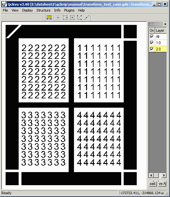
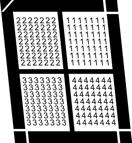
In order to show how the transformations work, we supply this simple GDSII file. We can then run it through the RIP with different transformation settings.

transform input file  500,000 x 610,000 um centered at 0,0

transform_test_case.gds 500,000 x 610,000 um centered at 0,0


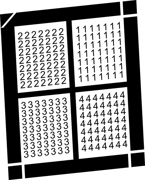
Rotation

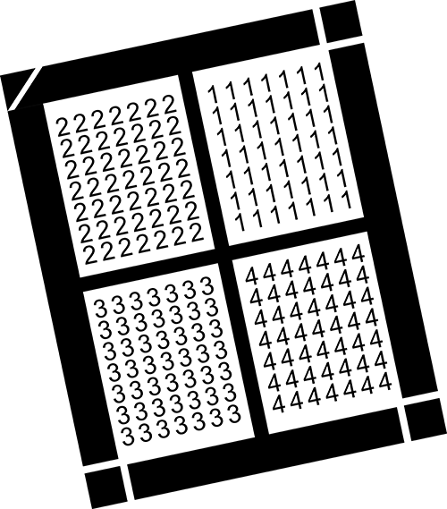
The output shown below has been rotated by 12 degrees. [Note that the data extents is increased by this transformation.]

plus_twelve_rotation.gif

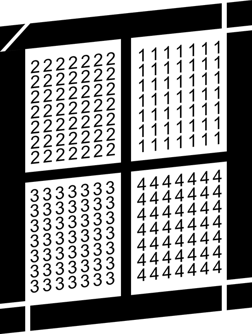
Mirror X

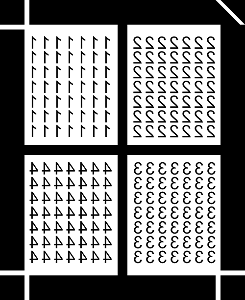
The output below has been set to Mirror X

mirror X

Mirror Y

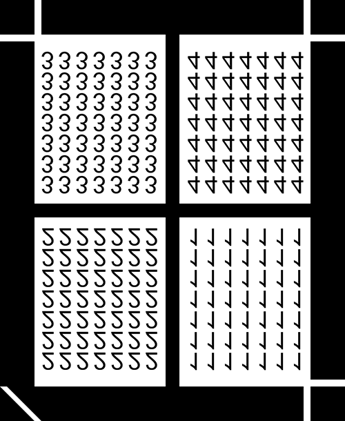
The output below has been set to Mirror Y

mirror Y

Scale (Y only)

The output is transformed by scaling the Y axis by 0.819.

scale transform X=1 Y=0.819

Shear (X only)

The output is transformed by setting ShearX = 6.

transform by shear X = 6

Shear (Y only)

The output is transformed by setting ShearY = 6.

transform ShearY=6

Shear X and Y

The output is transformed by setting ShearX = 3 and ShearY=6

Shea X set to 3 and ShearY set to 6


Tiles

A single large bitmap is often not useful. Therefore the program allows the user to define one or more (typically more than one) "tiles." Each tile covers a portion of the entire image area.

Manual Tile Assignment

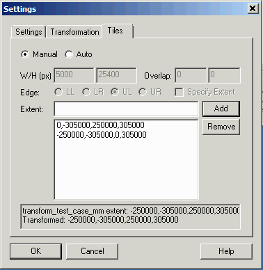
If Manual is selected, then the user can define one or more tiles areas by specifying the extents of the data that the tile should cover. This is made more complicated by the fact that the use must take into account any changes to the extents which were produced by transformations.

The program assists the user by presenting both the initial extents of the data and the transformed extents.

two_manual_tiles_dialog.gif

In the example dialog above, the user has specified two tiles. The first covers the left had side of the layout and the second covers the right hand side of the database. When this is rasterized, the results will be two separate tiles as shown below:

manual_tile1.gif

Automatic Tiling

When Automatic tiling is selected, the user specifies both the tile size and any overlap. The program will generate the tiles positions automatically to cover the extents it has been provided.

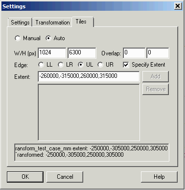
For example, assume our equipment wants to see bitmaps that are 1024 pixels wide and the whole height of the image. If our maximum image are is 630 mm x 520 mm and our pixel size = 100 um then we would define our tile size to be 1024 x 6300.

We also must decide on a reference corner -- in this case let us set the reference at the upper left of the

image area.

The dialog box would look like this:

tile_auto_example1.gif

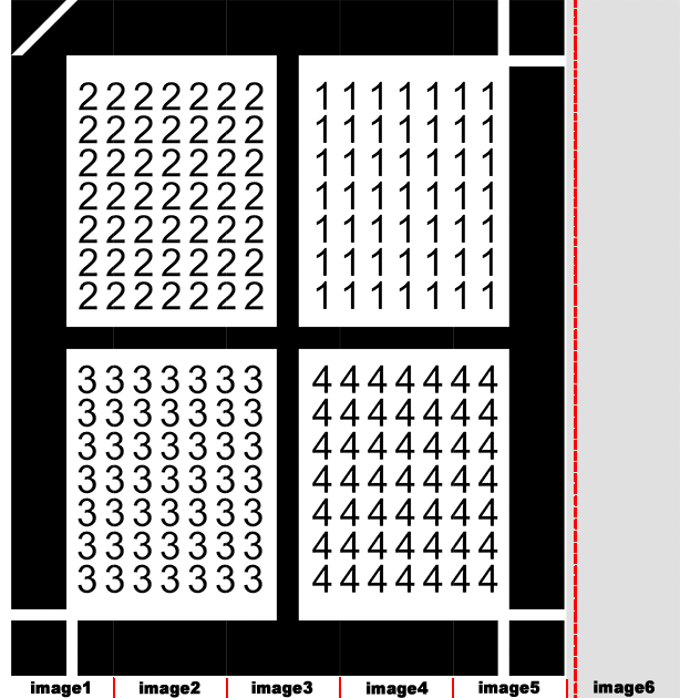
And the results would be 6 tiles arranged like this.

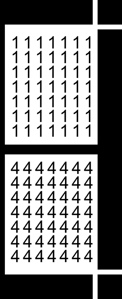
representation of how tiles are generated in auto mode

Notes:

Each tile is 1024 pixels wide by 630 pixels tall as specified.

Our tiling starting point was set to the upper left corner.

The final tile, tile6.tif, is "empty" because the the portion of it that covered the data was empty.


Span Length

Span length is a parameter used by QckRip to more efficiently process layouts that have a large number of small repeating elements.

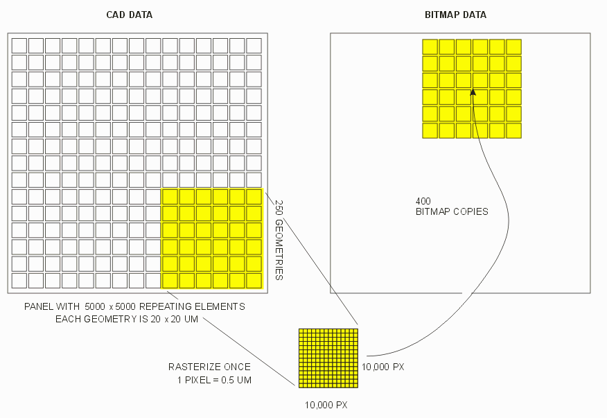
Consider a panel layout that has 5000 x 5000 small geometries on the order of 20 x 20 um in size. Without the span length operation, QckRip would create a bitmap of 20 x 20 um (at a pixel size of say 0.5 um) and use a bitmap copy operation 25 million times on a bitmap of only 1600 pixels.
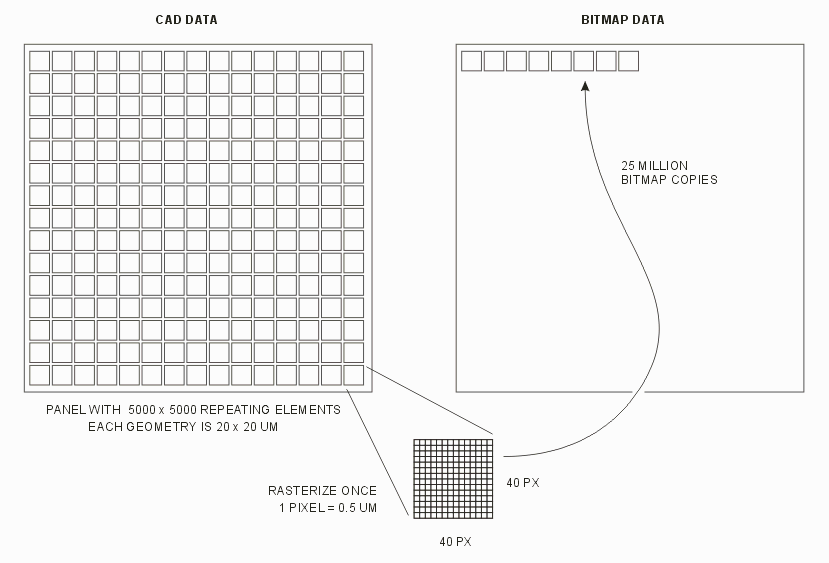
span_length1.gif

From a computational point of view this is not the most efficient approach - there are various computational costs to each bitmap copy that add up. With 25 million bitmap copies, even a small amount of overhead adds up.

It turns out that it would be much faster to spend a little more time up front and combine say, 250 x 250 of these tiny elements into a "super-block" -- a single geometry covering 5,000 x 5,000 um, rasterize that into a single bitmap of 100 megapixels, and then do a bitmap copy only 400 times.
span_length2.gif

Basically we are trading off some up front computation to combine and rasterize a larger area against time spent on a large number of bitmap copies.

Unfortunately it is not easy to predict the optimal size of the super block. It will depend on the complexity and hierarchy of the layout, the overall size of the layout and so on.

The span length entered by the user is an estimate of the super-block size; i.e. the length of an edge.


What are the limitations on setting the span length?

On the low side setting it to a value smaller than the smallest repeating geometry size essentially results in no creation of a super-block. In our example above, the repeating geometry is 20 x 20 um. So any span length less than 20 um does not result in creating a super block.

In practice such small values are ignored by the program and the value is set to an internal minimum.

On the high side you do not want the span length to exceed the extents of your repeating data -- again you will not get a repeating super-block. In our example above the layout is 100,000 um on a side so any setting above 100,000 um is also not helpful.

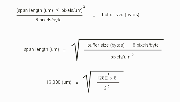
Also on the high side, the span length should not be set to produce a super-block whose bitmap cannot fit into the raster buffer. Say for our example we have a raster buffer size of 128 MB and our pixel size = 0.5 um.
span_length3.gif

the absolute maximum span length would be 16,000 um.

Even though the max allowed value for span length is constrained by the raster buffer size it is generally not helpful to select a span length so large.

As a starting point one should select a span length that is between 25% and 30% of the smaller of:

    a) the layout extents

    b) the raster buffer size limit (by converting back to an area based on the DPI)

In our example above the layout extents are 100,000 x 100,000 um which would give us a starting point for span length of of 25,000 to 30,000 um. The raster buffer is 128 MB which yields a max span length of 16,000 um. So this would give a starting point of 4000 to 5300 um. Since this is the smaller value one should start in the range of 4000 to 5000 um.